ClickHouse 10.数据查询

clickhouse

发布日期: 2021-07-10

1. 介绍

clickhouse 对 SQL 语句的解析时大小写敏感的，这就意味这，select a 和 select A 表达的语义是不同的
clickhouse 支持的查询语法如下：


[with expr | ( subquery ) ] 
select [ distinct ] expr
[ from [ db. ]table | ( subquery ) | table_function ] [ final ]
[ sample expr ]
[ [ left ] array join ]
[ global ]
[ all | any | asof ]
[ inner | cross | [ left | right | full [ outer ] ] ] join ( subquery ) | table on | using columns_list
[ prewhere expr ]
[ where expr ]
[ group by expr ]
[ with rollup | cube | totals ]
[ having expr ]
[ order by expr ]
[ limit [ n [ ,m ] ] ]
[ union all ]
[ into outfile finename ]
[ format format ]
[ limit [ offset ] n by columns ]

// 方括号内的查询子句为可选项，所以只有 select 子句是必须的
// clickhouse 对查询语法的解析大致也是按照上面各个子句排列的顺序进行的
// 下面介绍查询语法时也会按照上面的顺序进行介绍

2. with 子句

2.1 介绍

clickhouse 支持公共表表达式（CTE, Common Table Expressions）以增强查询语句的表达，如：

-- power(x, y) 接受x和y两个参数，返回x的y次方
select pow(pow(2,2),3) as result;

┌─result─┐
│     64 │
└────────┘

-- 改用 CTE 形式

WITH pow(2, 2) AS a
SELECT pow(a, 3) AS result;

┌─result─┐
│     64 │
└────────┘

CTE 通过 with 子句表示，还支持下面几种用法

2.2 定义变量

可以定义变量，这些变量在后面查询中能够直接被访问。

WITH 5 AS end
SELECT 
  number
FROM system.numbers
WHERE number < 5
LIMIT 3;

┌─number─┐
│      0 │
│      1 │
│      2 │
└────────

2.3 调用函数

可以访问 select 子句中的列字段，并调用函数做进一步的处理。

--  函数嵌套形式查询
SELECT
    database,
    formatReadableSize(sum(data_uncompressed_bytes) ) AS format
FROM system.columns
GROUP BY database
ORDER BY format DESC;

┌─database──────────┬─format────┐
│ system            │ 1.92 GiB  │
│ db1               │ 0.00 B    │
│ db2               │ 0.00 B    │
│ db_merge          │ 0.00 B    │
│ default           │ 0.00 B    │
│ db_Dictionary     │ 0.00 B    │
│ test_dictionaries │ 0.00 B    │
└───────────────────┴───────────┘

-- 改用 CTE 形式
WITH sum(data_uncompressed_bytes) AS bytes
SELECT
    database,
    formatReadableSize(bytes) AS format
FROM system.columns
GROUP BY database
ORDER BY bytes DESC;

┌─database──────────┬─format────┐
│ system            │ 1.92 GiB  │
│ db1               │ 0.00 B    │
│ db2               │ 0.00 B    │
│ db_merge          │ 0.00 B    │
│ default           │ 0.00 B    │
│ db_Dictionary     │ 0.00 B    │
│ test_dictionaries │ 0.00 B    │
└───────────────────┴───────────┘

2.4 定义子查询

-- 查询字段最多的三张表，以及占所有字段的百分比

WITH
    (
       SELECT 
          count(1)
       FROM system.columns
    ) AS total_columns
SELECT
    table,
    count(table) AS columns_count,
    (count(table) / total_columns) * 100 AS column_rate
FROM system.columns
GROUP BY table
ORDER BY column_rate DESC
LIMIT 3;

┌─table──────┬─columns_count─┬────────column_rate─┐
│ metric_log │           272 │ 21.829855537720707 │
│ query_log  │            62 │  4.975922953451043 │
│ parts      │            51 │  4.093097913322633 │
└────────────┴───────────────┴────────────────────┘


-- 注意 with 在使用子查询时只能返回一行数据，如果结果集大于 1 则会抛出异常

2.5 在子查询中重复使用 with

可以在子查询中嵌套使用 with 子句


with (
  round(column_rate) -- 对字段占比取整
) as column_rate_v1
select 
  table,
  columns_count,
  column_rate,
  column_rate_v1 
from (
  WITH ( -- 嵌套 with 
    SELECT 
    count(1)
    FROM system.columns
  ) AS total_columns
  SELECT
    table,
    count(table) AS columns_count, -- 计算每张表的字段数量
    (count(table) / total_columns) * 100 AS column_rate -- 计算字段数量占总量的比重
  FROM system.columns
  GROUP BY table
  ORDER BY column_rate DESC
  LIMIT 3
);

┌─table──────┬─columns_count─┬────────column_rate─┬─column_rate_v1─┐
│ metric_log │           272 │ 21.829855537720707 │             22 │
│ query_log  │            62 │  4.975922953451043 │              5 │
│ parts      │            51 │  4.093097913322633 │              4 │
└────────────┴───────────────┴────────────────────┴────────────────┘

3. from 子句

from 子句表示从何处读数据

-- 1. 从数据表读取数据

select name from system.columns limit 3;

┌─name───────────┐
│ department_id  │
│ employee_count │
│ salary_count   │
└────────────────┘

-- 2. 从子查询读取数据
select 
  name 
from (
  select name from system.columns limit 3
) ;

┌─name───────────┐
│ department_id  │
│ employee_count │
│ salary_count   │
└────────────────┘

-- 2. 从表函数中读取数据
select number from numbers(3);
┌─number─┐
│      0 │
│      1 │
│      2 │
└────────┘

from 关键字合一省略，此时会从续表中取数据，在 clickhouse 中并没有数据库中常见的 dual 虚表，而是用 system.one

-- 下面两个 SQL 是等价的
select 1;

┌─1─┐
│ 1 │
└───┘

select 1 from system.one;

┌─1─┐
│ 1 │
└───┘

from 子句后面可以使用 final 修饰符。它可以配合 collapsingMergeTree 和 Versioned-CollapsingMergeTree 等表引擎进行查询操作，以强制查询过程中合并，但是由于 final 修饰符会降低查询性能，所以应该尽可能避免使用它。

4. sample 子句

4.1 介绍

Sample 子句能够实现数据采样的功能，查询仅返回采样数据而不是全部数据，从而减少查询负载。
Sample 子句的采样机制是一种幂等的设计，在数据不发声变化的情况下，相同的规则返回的数据时相同的。
Sample 子句适合在可以接收近似查询结果的场合下使用，例如数据量巨大，对查询的实效性要求大于准确性的情况。
Sample 子句只能用于 MergeTree 表达式，并且建表时需要声明 sample by 抽样表达式。
使用示例

create table t_sample(
  id UInt8,
  name String,
  date DateTime
) engine = MergeTree()
partition by toYYYYMM(date)
order by (id,intHash32(id))
-- 采样键声明的表达式必须也包含在主键的声明中
-- 采样键必须是 Int 类型，否则在建表时会抛出异常
sample by intHash32(id);
-- 按照 intHash32(id) 分布后的结果采样查询


// 写入数据
insert into t_sample values(1,'小明','2021-06-26 11:40:41');
insert into t_sample values(2,'小红','2021-06-26 11:40:42');
insert into t_sample values(3,'小刚','2021-06-26 11:40:43');
insert into t_sample values(4,'小东','2021-06-26 11:40:44');
insert into t_sample values(5,'小丽','2021-06-26 11:40:45');

4.2 sample factor

sample factor 表示按照因子系数采样，其中 factor 表示采样因子，它的取值支持 0-1 之间的小数，如果 factor 设置为 0 或者 1 则效果等同于不进行采样。

-- 按照 40% 进行采样
select id,name from t_sample sample 0.4;

┌─id─┬─name─┐
│  1 │ 小明 │
│  3 │ 小刚 │
└────┴──────┘

-- 等同于 
select id,name from t_sample sample 40 / 100;

在进行统计查询时，为了得到最终的近似结果，需要将得到的直接结果乘以采样系数，若想要按 0.4 的因子采样，则需要将统计结果放大十倍。

select count(1) * 10 as sample from t_sample sample 0.4;
┌─sample─┐
│     20 │
└────────┘

还有一种方法是借助虚拟字段 _sample_factor 来获取采样稀疏，并以此代替硬编码的形式，_sample_factor 可以返回当前查询多对应的采样系数。

select id,_sample_factor from t_sample sample 0.4;

┌─id─┬─_sample_factor─┐
│  1 │            2.5 │
│  3 │            2.5 │
└────┴────────────────┘

-- 在使用_sample_factor 之后，可以将之前的查询语句改写成如下形式：
select count(1) * any(_sample_factor) from t_sample sample 0.4;

┌─multiply(count(), any(_sample_factor))─┐
│                                      5 │
└────────────────────────────────────────┘

4.3 sample rows

sample rows 是按照数量采样，其中 rows 表示至少采样多少行数据，它的取值必须是大于 1，如果 rows 的取值大于表内的总行数，则效果等于1 即不采样。
sample rows 采样数量的最小粒度是由 index_granularity 索引粒度决定的，所以设置一个小于索引粒度或者较小的值是没什么意义的，应该设置以为稍大的值。
sample rows 采样同样可以使用 _sample_factor 来获取当前查询所对应的采样系数。

select id,_sample_factor from t_sample sample 10000 limit 1;
┌─id─┬─_sample_factor─┐
│  1 │              1 │
└────┴────────────────┘

4.4 sample factor offset n

sample factor offset n 表示按照因子系数和偏移量采样，其中 factor 表示采样因子，n 表示便宜多少数据后才进行 CIA杨，他们的取值都是 0-1 之间的小数。

-- 设置采样系数为 0.4 偏移量为 0.2

select id,name from t_sample sample 0.4 offset 0.5;

┌─id─┬─name─┐
│  5 │ 小丽 │
└────┴──────┘

-- 上述代码表示查询会从二分之一的位置开始，按照 0.4 的系数采样
-- 如果计算 offset 偏移量之后，按照 sample 比例采样出现了溢出，则数据会被截断

5. array join 子句

5.1 介绍

array join 子句允许在数据表的内部与数组或嵌套类型的字段进行 join 操作，从而进行一行数据组展开为多行。
在一条 select 语句中，不使用子查询的情况下，只能存在一个 array join 子句，
array join 子句支持 inner 和 left 两种策略

-- 创建测试表

create table t_array_join(
  title String,
  value Array(UInt8)
) ENGINE= Log;

-- 写入测试数据
insert into t_array_join values
('food',[1,2,3]),
('fruit',[3,4]),
('meat',[]);

drop table t_array_join;

5.2 inner array join

array join 在默认情况下，使用的是 inner join 策略

select title,value from t_array_join array join value;

┌─title─┬─value─┐
│ food  │     1 │
│ food  │     2 │
│ food  │     3 │
│ fruit │     3 │
│ fruit │     4 │
└───────┴───────┘

-- 查询后可以发现，数据最终基于 value 被展开成了多行，并且排除了空数组，
-- 如果为原有数组字段添加一个别名，则能够访问展开前的数组字段

select title,value,v from t_array_join array join value as v;

┌─title─┬─value───┬─v─┐
│ food  │ [1,2,3] │ 1 │
│ food  │ [1,2,3] │ 2 │
│ food  │ [1,2,3] │ 3 │
│ fruit │ [3,4]   │ 3 │
│ fruit │ [3,4]   │ 4 │
└───────┴─────────┴───┘

5.3 left array join

-- left array join 示例
select title,value from t_array_join left array join value;

┌─title─┬─value─┐
│ food  │     1 │
│ food  │     2 │
│ food  │     3 │
│ fruit │     3 │
│ fruit │     4 │
│ meat  │     0 │ -- 因为 meat 行为空数组，查询时给出默认值
└───────┴───────┘

select title,value,v from t_array_join left array join value as v;

┌─title─┬─value───┬─v─┐
│ food  │ [1,2,3] │ 1 │
│ food  │ [1,2,3] │ 2 │
│ food  │ [1,2,3] │ 3 │
│ fruit │ [3,4]   │ 3 │
│ fruit │ [3,4]   │ 4 │
│ meat  │ []      │ 0 │
└───────┴─────────┴───┘
-- 在 left array join 中会把 inner join 中排除的空数组查询出来

当同时对多个数组字段进行 array join 操作时，查询的计算逻辑是按照行进行合并而不是产生笛卡尔积

SELECT
    title,
    value,
    v,
    arrayMap(x -> (x * 2), value) AS mapv,
    v1
FROM t_array_join
LEFT ARRAY JOIN
    value AS v,
    mapv AS v1;

┌─title─┬─value───┬─v─┬─mapv────┬─v1─┐
│ food  │ [1,2,3] │ 1 │ [2,4,6] │  2 │
│ food  │ [1,2,3] │ 2 │ [2,4,6] │  4 │
│ food  │ [1,2,3] │ 3 │ [2,4,6] │  6 │
│ fruit │ [3,4]   │ 3 │ [6,8]   │  6 │
│ fruit │ [3,4]   │ 4 │ [6,8]   │  8 │
│ meat  │ []      │ 0 │ []      │  0 │
└───────┴─────────┴───┴─────────┴────┘

-- value 和 mapv 数组是按行合并的，但是并没有产生笛卡尔积

在介绍数据类型时说过，嵌套类型的本质是数组，所以 arrau join 也支持嵌套类型的数据，

-- 建表
create table t_array_join_nested(
  title String,
  nest Nested(
    v1 UInt32,
    v2 UInt64
  )
) ENGINE= Log;

-- 写入数据
insert into t_array_join_nested values
('food',[1,2,3],[10,20,30]),
('fruit',[4,5],[40,50]),
('meat',[],[]);

-- 查询数据
select title,nest.v1,nest.v2 from t_array_join_nested array join nest.v1,nest.v2;
┌─title─┬─nest.v1─┬─nest.v2─┐
│ food  │       1 │      10 │
│ food  │       2 │      20 │
│ food  │       3 │      30 │
│ fruit │       4 │      40 │
│ fruit │       5 │      50 │
└───────┴─────────┴─────────┘

-- 也可以展开嵌套类型部分数据
select title,nest.v1,nest.v2 from t_array_join_nested array join nest.v1;

┌─title─┬─nest.v1─┬─nest.v2────┐
│ food  │       1 │ [10,20,30] │
│ food  │       2 │ [10,20,30] │
│ food  │       3 │ [10,20,30] │
│ fruit │       4 │ [40,50]    │
│ fruit │       5 │ [40,50]    │
└───────┴─────────┴────────────┘

-- 使用别名展开嵌套类型的数据同时查看原始数据
select title,nest.v1,v1_1,nest.v2,v2_1 from t_array_join_nested array join nest.v1 as v1_1,nest.v2 as v2_1;
┌─title─┬─nest.v1─┬─v1_1─┬─nest.v2────┬─v2_1─┐
│ food  │ [1,2,3] │    1 │ [10,20,30] │   10 │
│ food  │ [1,2,3] │    2 │ [10,20,30] │   20 │
│ food  │ [1,2,3] │    3 │ [10,20,30] │   30 │
│ fruit │ [4,5]   │    4 │ [40,50]    │   40 │
│ fruit │ [4,5]   │    5 │ [40,50]    │   50 │
└───────┴─────────┴──────┴────────────┴──────┘

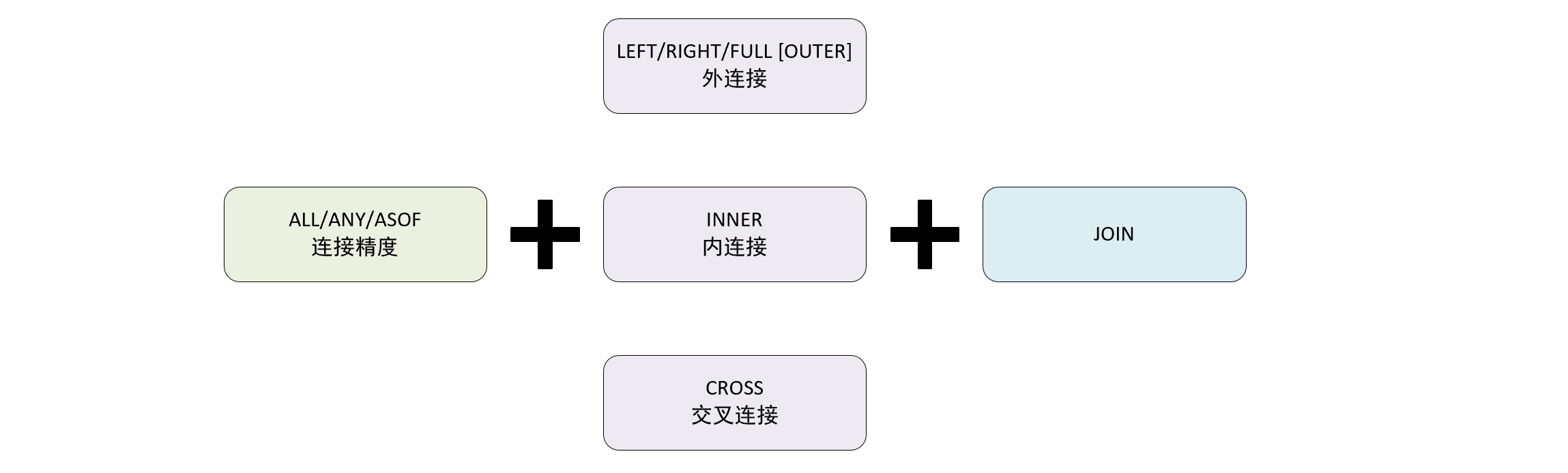
6. join 子句

6.1 介绍

join 子句可以对左右两张表的数据进行连接，它的语法包含连接精度和连接类型两个部分。

连接精度分为： all、any、asof 三种
连接类型分为：外连接、内连接、交叉连接三种
join 查询根据执行策略也可以被划分为本地查询和远程查询
准备数据

-- 创建表
create table t_join1(
  id String,
  name String,
  time DateTime
) ENGINE= Log;


-- 写入数据
insert into t_join1 values
('1','clickhouse','2021-07-12 16:50:01'),
('2','spark','2021-07-12 16:50:02'),
('3','es','2021-07-12 16:50:03'),
('4','hbase','2021-07-12 16:50:04'),
('','clickhouse','2021-07-12 16:50:05'),
('','spark','2021-07-12 16:50:06');

-- 创建表
create table t_join2(
  id String,
  rate UInt8,
  time DateTime
) ENGINE= Log;



-- 写入数据
insert into t_join2 values
('1','100','2021-07-12 16:50:01'),
('1','95','2021-07-12 16:50:01'),
('2','90','2021-07-12 16:50:02'),
('3','80','2021-07-12 16:50:03'),
('4','70','2021-07-12 16:50:04'),
('5','60','2021-07-12 16:50:05'),
('6','50','2021-07-12 16:50:06');

-- 创建表
create table t_join3(
  id String,
  star UInt8
) ENGINE= Log;

-- 写入数据
insert into t_join3 values
('1','1000'),
('2','900');

6.2 连接精度

连接精度决定了 join 查询在连接数据时所使用的的策略，目前支持 all，any 和 asof 三种，默认 all，还可以通过 join_default_strictness 配置默认参数修改默认的连接精度类型。

对于数据是否连接匹配的判断是通过 join key 进行的，目前只支持等式（equal join）。

交叉连接不需要使用 join key，因为它会产生笛卡尔积。

6.2.1 all

如果左表内的一行数据，在右表中存在多行数据与之连接匹配，则返回右表中全部连接的数据。
判断连接匹配的依据是左表与右表的数据，基于连接件（join key）的取值完全相等

SELECT
    t1.id,
    t1.name,
    t2.rate
FROM t_join1 AS t1
ALL INNER JOIN t_join2 AS t2 
ON t1.id = t2.id;

┌─id─┬─name───────┬─rate─┐
│ 1  │ clickhouse │ 100  │
│ 1  │ clickhouse │ 95   │
│ 2  │ spark      │ 90   │
│ 3  │ es         │ 80   │
│ 4  │ hbase      │ 70   │
└────┴────────────┴──────┘

-- 返回左右两张表中所有能够通过 id 匹配上的数据

6.2.2 any

如果左表的一行数据，在右表有多行与之连接匹配，则返回右表中的第一行数据。

SELECT
    t1.id,
    t1.name,
    t2.rate
FROM t_join1 AS t1
ANY INNER JOIN t_join2 AS t2 
ON t1.id = t2.id;

┌─id─┬─name───────┬─rate─┐
│ 1  │ clickhouse │ 100  │
│ 2  │ spark      │ 90   │
│ 3  │ es         │ 80   │
│ 4  │ hbase      │ 70   │
└────┴────────────┴──────┘
-- 仅返回左右两张表中能够匹配到的第一行数据

6.2.3 asof

asof 是一种模糊连接，它允许在连接件之后追加一个定义模糊连接的匹配条件 asof_column

SELECT
    t1.id,
    t1.name,
    t2.rate,
    t1.time,
    t2.time
FROM t_join1 AS t1
asof inner JOIN t_join2 AS t2 
ON 
  t1.id = t2.id 
and 
  t1.time >= t2.time;
  
-- 其中 ‘t1.id = t2.id ’ 为正常的连接键
-- ‘t1.time >= t2.time’ 为模糊键

┌─id─┬─name───────┬─rate─┬────────────────time─┬─────────────t2.time─┐
│ 1  │ clickhouse │ 100  │ 2021-07-12 16:50:01 │ 2021-07-12 16:50:01 │
│ 2  │ spark      │ 90   │ 2021-07-12 16:50:02 │ 2021-07-12 16:50:02 │
│ 3  │ es         │ 80   │ 2021-07-12 16:50:03 │ 2021-07-12 16:50:03 │
│ 4  │ hbase      │ 70   │ 2021-07-12 16:50:04 │ 2021-07-12 16:50:04 │
└────┴────────────┴──────┴─────────────────────┴─────────────────────┘

-- 最终返回的结果进返回了右表中能够匹配的第一行数据

asof 还支持使用 using 的简写形式，using 后声明的最后一个字段会被自动转换成 asof_column 模糊连接条件

SELECT
    t1.id,
    t1.name,
    t2.rate,
    t1.time,
    t2.time
FROM t_join1 AS t1
asof inner JOIN t_join2 AS t2 
using(id,time);
┌─id─┬─name───────┬─rate─┬────────────────time─┬─────────────t2.time─┐
│ 1  │ clickhouse │ 100  │ 2021-07-12 16:50:01 │ 2021-07-12 16:50:01 │
│ 2  │ spark      │ 90   │ 2021-07-12 16:50:02 │ 2021-07-12 16:50:02 │
│ 3  │ es         │ 80   │ 2021-07-12 16:50:03 │ 2021-07-12 16:50:03 │
│ 4  │ hbase      │ 70   │ 2021-07-12 16:50:04 │ 2021-07-12 16:50:04 │
└────┴────────────┴──────┴─────────────────────┴─────────────────────┘

对于 asof_column 字段的使用还需要注意两点：

asof_column 必须是整数、浮点数、日期类型这类有序序列的数据类型
asof_column 不能是数据表内的唯一字段，即连接键和asof_column 不能是同一字段

6.3 连接类型

连接类型决定了 join 查询组合左右两个数据集要用的策略，他们所形成的的结果集是交集、并集、笛卡尔积或是其他形式。

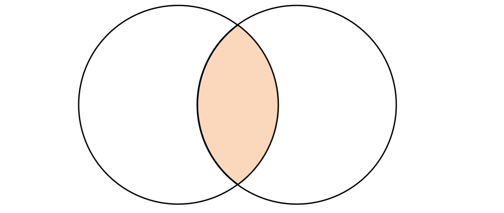
6.3.1 inner

inner 表示内连接，在查询时会以左表为基础逐行遍历数据，然后从由表中找出与左边连接的行，它只会返回左右两个数据集中交集的部分，其它部分都会被排除。

SELECT
    t1.id,
    t1.name,
    t2.rate
FROM t_join1 AS t1
INNER JOIN t_join2 AS t2 
ON t1.id = t2.id

┌─id─┬─name───────┬─rate─┐
│ 1  │ clickhouse │ 100  │
│ 1  │ clickhouse │ 95   │
│ 2  │ spark      │ 90   │
│ 3  │ es         │ 80   │
│ 4  │ hbase      │ 70   │
└────┴────────────┴──────┘

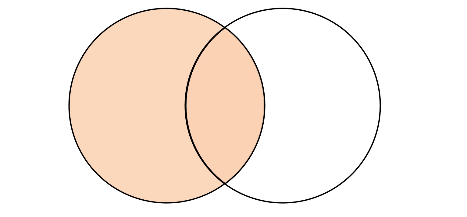
-- 左右两个数据集中，id 完全相同的数据才会保留，也就是只保留交集的部分

6.3.2 left [outer]

outer join 表示外连接，可以分为 left （左外连接），right（右外连接），full（全连接）三种形式，根据连接形式不同，返回的数据集合的逻辑也不相同。
在进行外连接查询时 outer 修饰符可以省略。
进行左外连接查询时，会以左表为基础，逐行遍历数据，然后从右表中找出与左边连接的行以补齐属性
如果右边没有找到连接的行，则采用响应字段数据类型的默认值填充

SELECT
    t1.id,
    t1.name,
    t2.rate
FROM t_join1 AS t1
LEFT JOIN t_join2 AS t2 ON t1.id = t2.id;

┌─id─┬─name───────┬─rate─┐
│ 1  │ clickhouse │  100 │
│ 1  │ clickhouse │   95 │
│ 2  │ spark      │   90 │
│ 3  │ es         │   80 │
│ 4  │ hbase      │   70 │
│    │ clickhouse │    0 │
│    │ spark      │    0 │
└────┴────────────┴──────┘

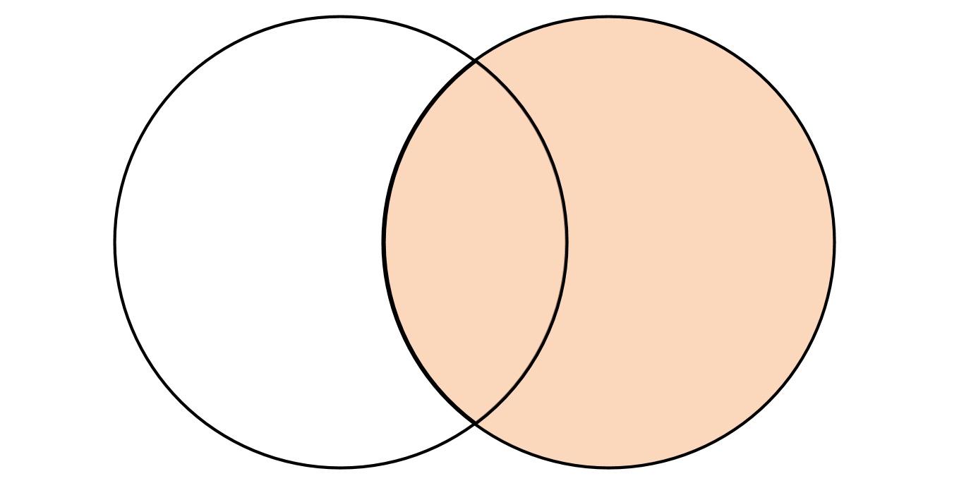
-- 返回 左表中的全部数据数据，其中当右表与左表没有关联上时，补充rate （UInt8 类型） 的默认值

6.3.3 right [outer]

右外连接跟左外连接的逻辑刚好相反，将右表的数据全部返回，而左表不能连接的数据使用默认值补全。
在内部进行 inner join 的内部连接查询，在计算交集部分的同时，顺便记录右表中有哪些数据未能被连接
将未能连接的数据行追加到交集的尾部
将追加数据的默认值补充到未能连接的数据中

SELECT
    t2.id,
    t1.name,
    t2.rate
FROM t_join1 AS t1
RIGHT JOIN t_join2 AS t2 ON t1.id = t2.id;

┌─t2.id─┬─name───────┬─rate─┐
│ 1     │ clickhouse │  100 │
│ 1     │ clickhouse │   95 │
│ 2     │ spark      │   90 │
│ 3     │ es         │   80 │
│ 4     │ hbase      │   70 │
└───────┴────────────┴──────┘
┌─t2.id─┬─name─┬─rate─┐
│ 6     │      │   50 │
│ 5     │      │   60 │
└───────┴──────┴──────┘

6.3.4 full [outer]

全外连接查询会返回左右两个数据集的并集。
全连接会在内部进行类似 left join 的查询，在左外连接的过程中，顺带记录由表中已经被连接的数据
通过在由表中记录已经被连接的数据得到未被连接的数据行，
将右表中未被连接的数据行追加至结果集，并将那些数据左表中的列字段以默认值补全。

SELECT
    t2.id,
    t1.name,
    t2.rate
FROM t_join1 AS t1
FULL JOIN t_join2 AS t2 ON t1.id = t2.id;

┌─t2.id─┬─name───────┬─rate─┐
│ 1     │ clickhouse │  100 │
│ 1     │ clickhouse │   95 │
│ 2     │ spark      │   90 │
│ 3     │ es         │   80 │
│ 4     │ hbase      │   70 │
│       │ clickhouse │    0 │
│       │ spark      │    0 │
└───────┴────────────┴──────┘
┌─t2.id─┬─name─┬─rate─┐
│ 6     │      │   50 │
│ 5     │      │   60 │
└───────┴──────┴──────┘

6.3.5 cross

cross join 表示交叉连接，它会返回左右两个数据集的笛卡尔积，也正是因为如此，cross join 不需要声明 join key，因为结果会包含他们所有的组合。
cross join 进行查询时，会以左表为基础，逐行与右表全集相乘。

SELECT
    t2.id,
    t1.name,
    t2.rate
FROM t_join1 AS t1
CROSS JOIN t_join2 AS t2;
┌─t2.id─┬─name───────┬─rate─┐
│ 1     │ clickhouse │  100 │
│ 1     │ clickhouse │   95 │
│ 2     │ clickhouse │   90 │
│ 3     │ clickhouse │   80 │
│ 4     │ clickhouse │   70 │
│ 5     │ clickhouse │   60 │
│ 6     │ clickhouse │   50 │
│ 1     │ spark      │  100 │
│ 1     │ spark      │   95 │
...
└───────┴────────────┴──────┘

6.4 多表连接

进行多张表的连接查询时，clickhouse 会将他们转为两两连接的形式，如下查询：


SELECT
    t2.id,
    t1.name,
    t2.rate,
    t3.star
FROM t_join1 AS t1
INNER JOIN t_join2 AS t2 ON t1.id = t2.id
LEFT JOIN t_join3 as t3 ON t1.id = t3.id;

┌─t2.id─┬─t1.name────┬─t2.rate─┬─t3.star─┐
│ 1     │ clickhouse │     100 │     232 │
│ 1     │ clickhouse │      95 │     232 │
│ 2     │ spark      │      90 │     132 │
│ 3     │ es         │      80 │       0 │
│ 4     │ hbase      │      70 │       0 │
└───────┴────────────┴─────────┴─────────┘

上面查询时，会先将 t_join1 与t_join2 进行内连接，之后再将其结果与 t_join3 进行左外连接。

-- 如果查询语句中不包含 where 条件，则会转换为 cross join 
SELECT
    t2.id,
    t1.name,
    t2.rate,
    t3.star
FROM t_join1 AS t1
, t_join2 AS t2
, t_join3 as t3;

┌─t2.id─┬─t1.name────┬─t2.rate─┬─t3.star─┐
│ 1     │ clickhouse │     100 │     232 │
│ 1     │ clickhouse │     100 │     132 │
│ 1     │ clickhouse │      95 │     232 │
│ 1     │ clickhouse │      95 │     132 │
│ 2     │ clickhouse │      90 │     232 │
│ 2     │ clickhouse │      90 │     132 │
│ 3     │ clickhouse │      80 │     232 │
│ 3     │ clickhouse │      80 │     132 │
│ 4     │ clickhouse │      70 │     232 │
│ 4     │ clickhouse │      70 │     132 │
│ 5     │ clickhouse │      60 │     232 │
│ 5     │ clickhouse │      60 │     132 │
│ 6     │ clickhouse │      50 │     232 │
│ 6     │ clickhouse │      50 │     132 │
...
└───────┴────────────┴─────────┴─────────┘

-- 如果查询语句中包含 where 条件，则会转换为 inner join 
SELECT
    t2.id,
    t1.name,
    t2.rate,
    t3.star
FROM t_join1 AS t1
, t_join2 AS t2
, t_join3 as t3 where t1.id = t2.id and t1.id = t3.id;

┌─t2.id─┬─t1.name────┬─t2.rate─┬─t3.star─┐
│ 1     │ clickhouse │     100 │     232 │
│ 1     │ clickhouse │      95 │     232 │
│ 2     │ spark      │      90 │     132 │
└───────┴────────────┴─────────┴─────────┘

6.5 注意事项

关于性能

为了能够优化 join 查询性能，应该遵循左大右小的原则，将数据量小的表放到右侧，因为无论是哪种连接方式，右表都会被全部加载到内存中与左表进行关联。
join 查询没有缓存的支持，这意味着，每一次 join 查询，即使是连续查询相同的 SQL 语句，也都会生成一次全新的执行计划，如果应用程序会大量使用 join 查询，则需要进一步考虑借助上层应用的缓存服务或使用 join 表引擎来改善性能。
如果是在大量纬度属性补全的场景中，建议使用字典代替 jion 查询，因为在进行多表连接查询时，查询会转换成两两连接的形式，这种方式的查询很可能带来性能问题

关于空值策略与简写形式

在之前进行的连接查询中，未关联上的数据会进行默认值补充，这与其他数据库采取的策略不同，连接查询的空值策略是通过 join_use_nulls 参数指定的，默认值是 0，当参数设置为 0 时，空值由数据类型的默认值补充，当设置为 1 时，空值由 null 补充。

Join key 支持简化写法，当表的连接字段名称相同时，可以使用 using 语法简写，如下：

SELECT
    t1.id,
    t1.name,
    t2.rate
FROM t_join1 AS t1
INNER JOIN t_join2 AS t2 
ON t1.id = t2.id

┌─id─┬─name───────┬─rate─┐
│ 1  │ clickhouse │ 100  │
│ 1  │ clickhouse │ 95   │
│ 2  │ spark      │ 90   │
│ 3  │ es         │ 80   │
│ 4  │ hbase      │ 70   │
└────┴────────────┴──────┘

-- 上面SQL 可以简写为
SELECT
    t1.id,
    t1.name,
    t2.rate
FROM t_join1 AS t1
INNER JOIN t_join2 AS t2 
using id;

┌─id─┬─name───────┬─rate─┐
│ 1  │ clickhouse │  100 │
│ 1  │ clickhouse │   95 │
│ 2  │ spark      │   90 │
│ 3  │ es         │   80 │
│ 4  │ hbase      │   70 │
└────┴────────────┴──────┘

7. where 和 prewhere 子句

where 子句基于条件表达式来实现数据过滤。如果过滤条件恰好是主键字段，则能够进一步借助索引加速查询，所以 where 子句是一条查询语句能够启用索引的判断依据（在表引擎支持索引的情况下），

select id,name,url from table where id = 'A000'

(SelectExecutor): Key condition:(column 0 in['A000' , 'A000'])

where 表达式中包含了主键，所以它能够使用索引过滤数据区间，除了 where 之外 clickhouse 还提供了 prewhere 子句。
prewhere 只能用于 MergeTree 系列的表引擎，可以看做是对 where 的一种优化，作用于 where 相同，均是用来过滤数据。
使用 prewhere 时，只会读取 prewhere 指定的字段，用于数据过滤的条件判断，过滤完成之后再读取 select 声明的字段补充其余属性，所以 prewhere 比 where 处理的数据量更少，效率更高。
在查询时 clickhouse 会自动优化，在合适的时候将 where 替换成 prewhere，（需要 SET optimize_move_to_prewhere = 1 ）

8. group by 子句

group by 又叫聚合查询，是最常用的子句之一
group by 后面声明的表达式通常称为聚合键，数据会按照聚合键进行聚合
clickhouse 聚合查询时，select 可以声明聚合函数和列字段，如果 select 后只声明了聚合函数，则可以省略 group by 关键字

SELECT
    sum(data_compressed_bytes) AS compressed,
    sum(data_uncompressed_bytes) AS uncompressed
FROM system.parts

┌─compressed─┬─uncompressed─┐
│  609726471 │  28057230433 │
└────────────┴──────────────┘

如果声明了列字段，则只能使用聚合键包含的字段，否则会报错

-- 除了聚合函数外，只能使用聚合key 中包含的 table 字段
select table,count(1)  FROM system.parts group by table;

-- 使用了聚合键之外的字段 row 则会报错
select table,rows,count(1)  FROM system.parts group by table;

在某些场合下可以借助 any,min,max 等集合函数来访问聚合键之外的列字段

select table,count(1),any(rows),min(rows),max(rows) from system.parts group by table;
┌─table────────────────┬─count()─┬─any(rows)─┬─min(rows)─┬─max(rows)─┐
│ t_sample             │       1 │         5 │         5 │         5 │
│ t_jbod               │       1 │       100 │       100 │       100 │
│ merge_column_ttl     │       1 │         2 │         2 │         2 │
│ metric_log           │     148 │   1340747 │         6 │   2136337 │
└──────────────────────┴─────────┴───────────┴───────────┴───────────┘

当聚合查询内的数据存在NULL 值时，clickhouse 会将 NULL 作为特定值处理

select arrayJoin([1,2,3,null,null]) as v group by v;
┌────v─┐
│    1 │
│    2 │
│    3 │
│ ᴺᵁᴸᴸ │
└──────┘

8.1 with rollup

rollup 能够按照聚合键从右向左上卷数据，基于聚合函数一次生成分组小计和总计。如果聚合键的个数为n 个，最终会生成小计的个数为 n+1 个。

select table,name,sum(bytes_on_disk) from system.parts group by table,name with rollup order by table;

┌─table──────────────────────────────────────────┬─name────────────────────────┬─sum(bytes_on_disk)─┐
│ t_merge_replace                                │                             │                482 │
│ t_merge_replace                                │ 202107_3_3_0                │                229 │
│ t_merge_replace                                │ 202106_1_2_1                │                253 │
└────────────────────────────────────────────────┴─────────────────────────────┴────────────────────┘
-- 返回结果中，有总计的结果（所有分区占用磁盘总量），也有每个分区的小计结果（每个分区占用磁盘量）

8.2 with cube

cube 会像立方体模型一样，基于聚合键之间所有的组合生成小计信息，如果设置聚合键为 n ，则最终小计组合个数为 2 的 n 次方。

-- 统计 db_merge 中的 t_merge_replace 表占用磁盘数量，
-- 通过查询 system.parts 系统表，分别按照 database,table,name 分组合计汇总

select 
  database,
  table,
  name,
  sum(bytes_on_disk) 
from (
  select 
    database,
    table,
    name,
    bytes_on_disk from system.parts
  where table = 't_merge_replace'
) group by database,table,name
with cube
order by database,table,name;

┌─database─┬─table───────────┬─name─────────┬─sum(bytes_on_disk)─┐
│          │                 │              │                482 │
│          │                 │ 202106_1_2_1 │                253 │
│          │                 │ 202107_3_3_0 │                229 │
│          │ t_merge_replace │              │                482 │
│          │ t_merge_replace │ 202106_1_2_1 │                253 │
│          │ t_merge_replace │ 202107_3_3_0 │                229 │
│ db_merge │                 │              │                482 │
│ db_merge │                 │ 202106_1_2_1 │                253 │
│ db_merge │                 │ 202107_3_3_0 │                229 │
│ db_merge │ t_merge_replace │              │                482 │
│ db_merge │ t_merge_replace │ 202106_1_2_1 │                253 │
│ db_merge │ t_merge_replace │ 202107_3_3_0 │                229 │
└──────────┴─────────────────┴──────────────┴────────────────────┘

8.3 with totals

使用 totals 修饰符后，会基于聚合函数对所有数据进行汇总，

select database,sum(bytes_on_disk),count(table) from system.parts group by database with totals;

┌─database─┬─sum(bytes_on_disk)─┬─count(table)─┐
│ query    │                271 │            1 │
│ db1      │               1306 │            6 │
│ db_merge │               4856 │           15 │
│ system   │          635254433 │          192 │
│ default  │            3057737 │            2 │
└──────────┴────────────────────┴──────────────┘

Totals:
┌─database─┬─sum(bytes_on_disk)─┬─count(table)─┐
│          │          638318603 │          216 │
└──────────┴────────────────────┴──────────────┘

-- 结果中增加了一行 totals 汇总合计，这个结果是基于聚合函数所有数据聚合汇总的结果。

9. having

having 子句需要依赖 group by 使用，它能够在聚合计算之后实现二次过滤

-- 下面是一条按照 table 分区计数的聚合语句
EXPLAIN
SELECT 
  count(1)
FROM system.parts
GROUP BY database


┌─explain───────────────────────────────────────────────────────────────────────┐
│ Expression ((Projection + Before ORDER BY))                                   │
│   Aggregating                                                                 │
│     Expression (Before GROUP BY)                                              │
│       SettingQuotaAndLimits (Set limits and quota after reading from storage) │
│         ReadFromStorage (SystemParts)                                         │
└───────────────────────────────────────────────────────────────────────────────┘

-- 使用 having 子句将上面的聚合查询进行数据过滤， 
EXPLAIN
SELECT 
  count(1)
FROM system.parts
GROUP BY database
having table ='t_merge_replace'

┌─explain─────────────────────────────────────────────────────────────────────────┐
│ Expression ((Projection + Before ORDER BY))                                     │
│   Aggregating                                                                   │
│     Expression (Before GROUP BY)                                                │
│       Filter (WHERE)                                                            │
│         SettingQuotaAndLimits (Set limits and quota after reading from storage) │
│           ReadFromStorage (SystemParts)                                         │
└─────────────────────────────────────────────────────────────────────────────────┘

-- 可以看到 在聚合之后，增加了一步 filter 操作

-- 上述同样的操作还可以使用 where 条件实现
EXPLAIN
SELECT 
  count(1)
FROM
(
    SELECT 
      database
    FROM system.parts
    WHERE table = 't_merge_replace'
)
GROUP BY database

┌─explain─────────────────────────────────────────────────────────────────────────┐
│ Expression ((Projection + Before ORDER BY))                                     │
│   Aggregating                                                                   │
│     Expression ((Before GROUP BY + (Projection + Before ORDER BY)))             │
│       Filter (WHERE)                                                            │
│         SettingQuotaAndLimits (Set limits and quota after reading from storage) │
│           ReadFromStorage (SystemParts)                                         │
└─────────────────────────────────────────────────────────────────────────────────┘

-- 从执行计划可以看出使用 where 条件过滤的方式要比 having 效率更好，因为 where 的方式使用了谓词下推，聚合之前就过滤了大部分数据减少了要计算的数据量

having 子句经常用在我们要过滤聚合后的数据的情况，比如按照 table 聚合，过滤出聚合数值大于 1000000 字节的表

SELECT
    table,
    sum(bytes_on_disk) AS total
FROM system.parts
GROUP BY table
HAVING total > 1000000

┌─table───────────────────┬─────total─┐
│ metric_log              │ 606119816 │
│ t_hot_to_cold           │   3057506 │
│ asynchronous_metric_log │  31422436 │
└─────────────────────────┴───────────┘

10. order by

order by 子句通过声明排序键来指定查询数据返回时的顺序，在 mergeTree 表引擎中也有 order by 参数用于指定排序键，MergeTree 中指定排序键后，数据在各个分区内会按照定对的规则排序，这是一种分区内的局部排序，如果在查询时跨越了多个分区，则返回结果数据的顺序是未知的，每次查询结果可能都不相同，如果想对结果进行排序，就需要在查询时使用 order by 子句来实现全局排序。

order by 在使用时，可以定义多个排序键，每个排序键可以跟 ASC(升序)或 DESC(降序) 来确定排序顺序，如果不写则默认升序。

-- v1 升序，v2 降序
select arrayJoin([1,2,3]) as v1,arrayJoin([4,5,6]) as v2 order by v1 ASC,v2 DESC;
┌─v1─┬─v2─┐
│  1 │  6 │
│  1 │  5 │
│  1 │  4 │
│  2 │  6 │
│  2 │  5 │
│  2 │  4 │
│  3 │  6 │
│  3 │  5 │
│  3 │  4 │
└────┴────┘

-- v1 升序，v2 降序
select arrayJoin([1,2,3]) as v1,arrayJoin([4,5,6]) as v2 order by v1 ,v2 DESC;
┌─v1─┬─v2─┐
│  1 │  6 │
│  1 │  5 │
│  1 │  4 │
│  2 │  6 │
│  2 │  5 │
│  2 │  4 │
│  3 │  6 │
│  3 │  5 │
│  3 │  4 │
└────┴────┘

-- v1，v2 都降序
select arrayJoin([1,2,3]) as v1,arrayJoin([4,5,6]) as v2 order by v1 DESC ,v2 DESC;

┌─v1─┬─v2─┐
│  3 │  6 │
│  3 │  5 │
│  3 │  4 │
│  2 │  6 │
│  2 │  5 │
│  2 │  4 │
│  1 │  6 │
│  1 │  5 │
│  1 │  4 │
└────┴────┘

10.1 nulls last

NULL 值排在最后，这也是默认行为，修饰符可以省略，在这种情况下，数据排序为：其他值 > NaN > NULL

with arrayJoin([20,null,32.3,0/0,1/0,-1/0]) as v1
select v1
┌───v1─┐
│   20 │
│ ᴺᵁᴸᴸ │
│ 32.3 │
│  nan │
│  inf │
│ -inf │
└──────┘

with arrayJoin([20,null,32.3,0/0,1/0,-1/0]) as v1
select v1 order by v1 desc nulls last;
┌───v1─┐
│  inf │
│ 32.3 │
│   20 │
│ -inf │
│  nan │
│ ᴺᵁᴸᴸ │
└──────┘

-- 等同于
with arrayJoin([20,null,32.3,0/0,1/0,-1/0]) as v1
select v1 order by v1 desc;
┌───v1─┐
│  inf │
│ 32.3 │
│   20 │
│ -inf │
│  nan │
│ ᴺᵁᴸᴸ │
└──────┘

10.2 nulls first

NULL 值排在最前面，这情况下数据的排序顺序为：NULL > NaN > 其他值

with arrayJoin([20,null,32.3,0/0,1/0,-1/0]) as v1
select v1 order by v1 desc nulls first;

┌───v1─┐
│ ᴺᵁᴸᴸ │
│  nan │
│  inf │
│ 32.3 │
│   20 │
│ -inf │
└──────┘

11. limit by

limit by 子句和 limit 有所不同，它运行在 order by 之后和 limit 之前，能够按照指定分组，返回前 n 行数据，如果数据少于 n 行则按实际数量返回。
limit by 子句常用于 top N 场景。

-- 查询每个数据库中占用磁盘最多的三张表
SELECT
    database,
    table,
    sum(bytes_on_disk) AS bytes
FROM system.parts
GROUP BY
    database,
    table
ORDER BY
    database DESC,
    bytes DESC
LIMIT 2 BY database

┌─database─┬─table───────────────────┬─────bytes─┐
│ system   │ metric_log              │ 479773421 │
│ system   │ asynchronous_metric_log │  31669444 │
│ query    │ t_sample                │       271 │
│ default  │ t_hot_to_cold           │   3057506 │
│ default  │ insert_test             │       231 │
│ db_merge │ t_jbod                  │       779 │
│ db_merge │ t_merge_tree_partition  │       672 │
│ db1      │ t_partition             │       465 │
│ db1      │ t_partition_default     │       390 │
└──────────┴─────────────────────────┴───────────┘

声明多个表达式需要使用逗号分隔。

1	ORDER BY col1 DESC LIMIT 2 BY col1,col2

limit by 也支持跳过 offset 偏移量获取数据

limit n offset y by express
-- 或者
limit y,n by express

-- 查询结果跳过 1 行数据的位置开始
SELECT
    database,
    table,
    max(bytes_on_disk) AS bytes
FROM system.parts
GROUP BY
    database,
    table
ORDER BY bytes DESC
LIMIT 1, 3 BY database


┌─database─┬─table───────────────────┬───bytes─┐
│ system   │ asynchronous_metric_log │ 8388674 │
│ system   │ query_log               │  202273 │
│ system   │ query_thread_log        │  186276 │
│ db_merge │ t_merge_sum_nested      │     438 │
│ db_merge │ t_merge_sum             │     407 │
│ db_merge │ t_merge_agg             │     362 │
│ db1      │ t_partition             │     233 │
│ db1      │ t_partition_default     │     232 │
│ default  │ insert_test             │     231 │
│ db1      │ alter_add_column        │     218 │
└──────────┴─────────────────────────┴─────────┘

-- 不跳过 offset 查询数据示例
SELECT
    database,
    table,
    max(bytes_on_disk) AS bytes
FROM system.parts
GROUP BY
    database,
    table
ORDER BY bytes DESC
LIMIT 3 BY database

┌─database─┬─table───────────────────┬────bytes─┐
│ system   │ metric_log              │ 97797533 │ -- 这行数据在前一次查询中被跳过了
│ system   │ asynchronous_metric_log │  8388674 │
│ default  │ t_hot_to_cold           │  3057506 │
│ system   │ query_log               │   202273 │
│ db_merge │ t_jbod                  │      779 │
│ db_merge │ t_merge_sum_nested      │      438 │
│ db_merge │ t_merge_sum             │      407 │
│ query    │ t_sample                │      271 │
│ db1      │ t_partition_b           │      233 │
│ db1      │ t_partition             │      233 │
│ db1      │ t_partition_default     │      232 │
│ default  │ insert_test             │      231 │
└──────────┴─────────────────────────┴──────────┘

12. limit

limit 子句用于返回指定的前 n 行数据，常用于分页场景。

-- 返回前 你条数据
limit n
-- 从第 y 行数据开始，返回 n 条数据
limit n offset y
-- 从第 y 行数据开始，返回 n 条数据
limit y,n

-- 返回前 5 条数据
select number from system.numbers limit 5;
┌─number─┐
│      0 │
│      1 │
│      2 │
│      3 │
│      4 │
└────────┘

-- 从第 3 行数据开始 返回 5 条数据
select number from system.numbers limit 5 offset 3;
┌─number─┐
│      3 │ -- 跳过了 0，1，2 3 条数据
│      4 │
│      5 │
│      6 │
│      7 │
└────────┘

-- 同上
select number from system.numbers limit 3,5;
┌─number─┐
│      3 │
│      4 │
│      5 │
│      6 │
│      7 │
└────────┘

limit 子句可以和 limit by 一起使用

-- 不使用 limit 查询结果跳过 1 行数据的位置开始
SELECT
    database,
    table,
    max(bytes_on_disk) AS bytes
FROM system.parts
GROUP BY
    database,
    table
ORDER BY bytes DESC
LIMIT 1, 3 BY database

┌─database─┬─table───────────────────┬───bytes─┐
│ system   │ asynchronous_metric_log │ 8388674 │
│ system   │ query_log               │  202273 │
│ system   │ query_thread_log        │  186276 │
│ db_merge │ t_merge_sum_nested      │     438 │
│ db_merge │ t_merge_sum             │     407 │
│ db_merge │ t_merge_agg             │     362 │
│ db1      │ t_partition             │     233 │
│ db1      │ t_partition_default     │     232 │
│ default  │ insert_test             │     231 │
│ db1      │ alter_add_column        │     218 │
└──────────┴─────────────────────────┴─────────┘

-- 使用 limit 查询前 3 行数据， 查询结果跳过 1 行数据的位置开始
SELECT
    database,
    table,
    max(bytes_on_disk) AS bytes
FROM system.parts
GROUP BY
    database,
    table
ORDER BY bytes DESC
LIMIT 1, 3 BY database
LIMIT 3

┌─database─┬─table───────────────────┬───bytes─┐
│ system   │ asynchronous_metric_log │ 8388674 │
│ system   │ query_log               │  202273 │
│ system   │ query_thread_log        │  186276 │
└──────────┴─────────────────────────┴─────────┘

在使用 limit 查询数据跨越多个分区的时候，在没有是有 order by 进行全局排序的情况下，每次 limit 查询返回的数据可能有所不同，所以建议搭配 order by 一起使用。

13. select

select 子句决定了一次查询语句最终返回哪些字段或表达式，虽然 select 语句位于 SQL 语句的起始位置，但是它确实在一众句子之后执行的。在其它子句执行以后，select 会将选取的字段或表达式作用于每一行数据。
如果使用通配符 * 则返回数据表的所有字段，但是作为列式数据库的clickhouse，并不建议这么做。
clickhouse 还提供了基于正则表达式查询的形式

-- 查询以 n 开头的字段与包含 n 的字段

SELECT
    COLUMNS('^n'),
    COLUMNS('p')
FROM system.databases
LIMIT 2

┌─name─┬─data_path──────────────────┬─metadata_path───────────────────────────────────────────────────────┐
│ db1  │ /var/lib/clickhouse/store/ │ /var/lib/clickhouse/store/1b6/1b63d246-d32d-45f1-a6eb-553dde05598b/ │
│ db2  │ /var/lib/clickhouse/store/ │ /var/lib/clickhouse/store/47c/47c94419-6675-4861-a5f5-c76cb0b2acc2/ │
└──────┴────────────────────────────┴─────────────────────────────────────────────────────────────────────┘

14. distinct

distinct 子句能够去除重复数据

-- 创建测试表与测试数据

create table t_distinct(
  name String,
  value UInt8
)ENGINE=TinyLog;

insert into t_distinct values
('a',1),
('a',2),
('b',1),
('b',3),
('c',3);

select distinct name from t_distinct;

┌─name─┐
│ a    │
│ b    │
│ c    │
└──────┘

distinct 与 order by 比较

-- 使用 distinct 查询 ，查看 distinct 执行计划
EXPLAIN
SELECT DISTINCT name
FROM t_distinct;

┌─explain─────────────────────────────────────────────────────────────────────────┐
│ Expression (Projection)                                                         │
│   Distinct                                                                      │
│     Distinct (Preliminary DISTINCT)                                             │
│       Expression (Before ORDER BY)                                              │
│         SettingQuotaAndLimits (Set limits and quota after reading from storage) │
│           ReadFromStorage (TinyLog)                                             │
└─────────────────────────────────────────────────────────────────────────────────┘

-- 使用 group by 查询 ，查看 distinct 执行计划
EXPLAIN
SELECT name
FROM t_distinct
GROUP BY name;

┌─explain───────────────────────────────────────────────────────────────────────┐
│ Expression ((Projection + Before ORDER BY))                                   │
│   Aggregating                                                                 │
│     Expression (Before GROUP BY)                                              │
│       SettingQuotaAndLimits (Set limits and quota after reading from storage) │
│         ReadFromStorage (TinyLog)                                             │
└───────────────────────────────────────────────────────────────────────────────┘

distinct 与 group by 可以同时使用，如果使用了 limit 且没有 order by 子句，则 distinct 在满足条件时能够迅速结束查询，这样可以避免多余处理逻辑，当 distinct 与 group by 同时使用时，执行优先级是先 distinct 后 order by。

15. union all

union all 子句能够联合左右两边的两组查询，将结果合并一起返回，在一次查询中可以声明多次 union all 以便联合多组查询。
union all 子句两侧的查询必须做到字段数量和字段类型一致，否则无法将数据联合到一起，
union all 子句两侧的查询的字段名可以不同，查询结果会以左侧表的字段名为准

select name,value from t_distinct limit 2
union all
select name,value from t_distinct limit 2
union all
select name,value from t_distinct limit 2;

┌─name─┬─value─┐
│ a    │     1 │
│ a    │     2 │
└──────┴───────┘
┌─name─┬─value─┐
│ a    │     1 │
│ a    │     2 │
└──────┴───────┘
┌─name─┬─value─┐
│ a    │     1 │
│ a    │     2 │
└──────┴───────┘